
Graphical Analysis using ImageJ and Excel
In this page, results of several morphometric measurements are used to create scientific graphs through Excel.
1. Area and Roundness Distribution (Using ImageJ)
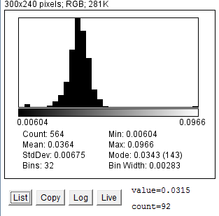

Figure 7. Area distribution of particles (red blood cells) in one image.
Figure 8. Roundness distribution of particles (red blood cells) in one image.
Under Analyse > Distribution, ImageJ has the ability to create simple distribution graphs, such as area distribution (Figure 7) and roundness distribution (Figure 8). Although this technique has many limitations, including the lack of a numbered x and y scale and the lack of an outline on each bar that separates them clearly, it is a quick and simple way of obtaining statistical analysis on results, including standard deviation, mean, min and max values.
2. Graphical Analysis of Area and Circularity (using Excel)
Although not a highly relevant section in this ImageJ Tutorial, this section shows some of the graphical analysis suitable to further the use of results obtained through ImageJ. And it signifies the ability of ImageJ to derive measurements that are only possible using image processing softwares, and illustrates how this can contribute to the scientific community.
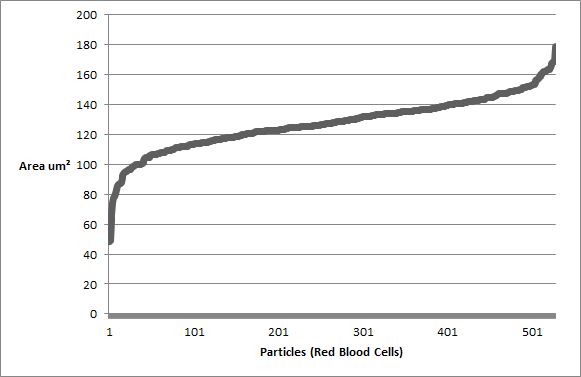
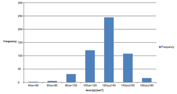
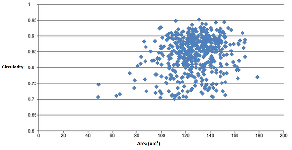
Figure 11: Circularity (y-axis) over Area (x-axis) of particles (red blood cells) in one image.
Figure 10: Frequency graph of the area of particles (red blood cells) in one image.
Figure 9: Particles (Red Blood Cells) arranged in ascending order based on their area.
To end this tutorial, here is a discussion of the findings shown on these graphs.
There is a gradual increase in particle (red blood cell) size in the majority of the middle part of figure 9. In addition, there is a steep increase in area at both the beginning and end of the graph (fig. 9). Since the particles were arranged in ascending order based on area, this suggests that particle area may follow a normal distribution. Figure 10 was created to test this, and as illustrated, a highly symmetrical normal distribution curve is created when an area frequency graph is generated. There are 2 particles in the 40-60 um^2 range (fig. 10) which results in a slightly negative skew in the graph. These two particles could however be outliers within the analysis that are not red blood cells but smaller fragments of red blood cells or background noise within the image that should have been excluded in the analysis. This, perhaps, shows one the key limitations of imagej, where any analysis is only as reliable as the image taken into the analysis. If, for example, the thresholding process, or image restriction process was not done adequately, a significant more amount of stray particles would have been included into the raw results. Even in this example, it is hard to determine whether these outliers are actually red blood cells or unrelated particle fragments. To continue, figure 11 shows that red blood cells are most clustered in a specific area and circularity value. As this specifc area and circularity value increases and decreases, the concentration of particles in the graph gradually declines in all directions. The position of the outliers in relation to all the other particles is shown as well; the relatively low value of circularity of outliers in the 40-60 um^2 range further suggests that they are possibly unrelated particle fragments instead of red blood cells.
References
Bankhead, Peter (2014) Analyzing fluorescence microscopy images with ImageJ [Online] Available from: http://blogs.qub.ac.uk/ccbg/files/2014/05/2014-05_Analyzing_fluorescence_microscopy_images.pdf [Accessed 24 May 2015]
Collins, T. J. (2007). ImageJ for microscopy. Biotechniques, 43(1 Suppl), 25-30.
Empix Imaging (2015) Northern Eclipse Help Reference – Object Parameters [Online] Available from: http://www.empix.com/NE%20HELP/functions/glossary/morphometric_param.html [Accessed 20 May 2015]
Foley, K (2014) Counting Cells with ImageJ [online video] Available from: https://www.youtube.com/watch?v=D1qBaFwuF4E [Accessed 16 November 2014]
Gelsvartas, J. (undated) Geometric Morphometrics [Online] Available from: http://homepages.inf.ed.ac.uk/rbf/CVonline/LOCAL_COPIES/AV0910/gelsvartas.pdf [Accessed 24 May 2015]
Ian, C (2014) Quantifying Stained Liver Tissue Area Using ImageJ[online video] Available from: https://www.youtube.com/watch?v=M8Eqq_nn4as [Accessed 20 November 2014]
ImageJ (2013) Particle Analysis [Online] Available from: http://imagej.net/Particle_Analysis [Accessed 24 May 2015]
IMSC (undated) IPSS ImageJ Hands-On Session 1: Image Segmentation [Online] Available from: http://www.lmsc.ethz.ch/Teaching/ipss_2010/TI_2_Longair_ [Accessed 24 May 2015]
Jensen, E.C. (2013), ‘Quantitative Analysis of Histological Staining and Fluorescence Using ImageJ’. Anat Rec, 296: 378–381.
Mcnaughton.A (2010) Measuring Area Using Thresholds [Online] Available from: http://occm.otago.ac.nz/resources/ImageJ-Thresholding.pdf [Accessed 24 May 2015]
Quantrachrome (2015) Feret Diameter [Online] Available from: http://www.quantachrome.co.uk/en/dictionary/Feret-diameter.asp [Accessed 24 May 2015]
Rohlf, F.J. (2015) Morphometrics [Online] Available from: http://life.bio.sunysb.edu/morph/ [Accessed 24 May 2015]
RSB (2015a) Introduction [Online] Available from: http://rsb.info.nih.gov/ij/docs/intro.html [Accessed 24 May 2015]
RSB (2015b) Quantifying Stained Liver Tissue [Online] Available from: http://rsbweb.nih.gov/ij/docs/examples/stained-sections/index.html [Accessed 24 May 2015]
RSB (2015c) Analyze Menu [Online] Available from: http://rsb.info.nih.gov/ij/docs/menus/analyze.html [Accessed 24 May 2015]